Lesson 15
Quartiles and Interquartile Range
15.1: Notice and Wonder: Two Parties (5 minutes)
Warm-up
In earlier lessons, students learned that the mean absolute deviation (MAD) is a measure of variability. In this warm-up, they study two distributions that appear very different but turn out to have the same MAD. Students notice that the MAD may not fully tell us about the variability of a data set. The work here motivates the need to have a different way to quantify variability, which is the focus of this lesson. While students may notice and wonder many things about these images, highlight ideas related to the variability of the data sets.
Launch
Arrange students in groups of 2. Display the dot plots for all to see. Ask students to identify at least one thing they notice and at least one thing they wonder about the dot plots, and to give a signal when they have both. Give students 1 minute of quiet think time, and then 1 minute to discuss their observation and question with their partner. Follow with a whole-class discussion.
Student Facing
Here are dot plots that show the ages of people at two different parties. The mean of each distribution is marked with a triangle.
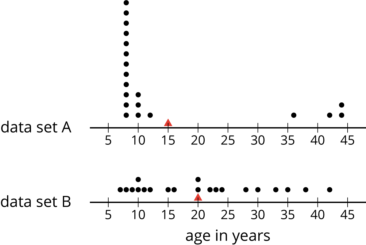
What do you notice and what do you wonder about the distributions in the two dot plots?
Student Response
For access, consult one of our IM Certified Partners.
Activity Synthesis
Invite students to share what they noticed and wondered. Record and display their responses for all to see. If possible, record the relevant reasoning on or near the image. After each response, ask the class if they agree or disagree and to explain alternative ways of thinking, referring back to the dot plots each time. Discuss:
- “Do you think the ages of the people at the first party are alike or different? What about the ages of the people at the second party?”
- “The MAD for both data sets is approximately 10.5 years. What does a MAD of 10.5 years tell us in this context?”
- “Is the MAD a useful description of variability in the first data set? What about in the second data set?”
Two key ideas to uncover here are:
- The MAD is a way to summarize variation from the mean, but the single number does not always tell us how the data are distributed.
- The same MAD could result from very different distributions.
If the key ideas above are not uncovered during discussion, be sure to highlight them.
15.2: The Five-Number Summary (15 minutes)
Activity
This activity introduces students to the five-number summary and the process of identifying the five numbers. Students learn how to partition the data into four sets: using the median to decompose the data into upper and lower halves, and then finding the middle of each half to further decompose it into quarters. They learn that each value that decomposes the data into four parts is called a quartile, and the three quartiles are the first quartile (Q1), second quartile (Q2, or the median), and third quartile (Q3). Together with the minimum and maximum values of the data set, the quartiles provide a five-number summary that can be used to describe a data set without listing or showing each data value.
Students reason abstractly and quantitatively (MP2) as they identify and interpret the quartiles in the context of the situation given.
Launch
Explain to students that they previously summarized variability by finding the MAD, which involves calculating the distance of each data point from the mean and then finding the average of those distances. Explain that we will now explore another way to describe variability and summarize the distribution of data. Instead of measuring how far away data points are from the mean, we will decompose a data set into four equal parts and use the markers that partition the data into quarters to summarize the spread of data.
Remind students that when there is an even number of values, the median is the average of the middle two values.
Arrange students in groups of 2. Give groups 8–10 minutes to complete the activity. Follow with a whole-class discussion.
Student Facing
Here are the ages of the people at one party, listed from least to greatest.
- 7
- 8
- 9
- 10
- 10
- 11
- 12
- 15
- 16
- 20
- 20
- 22
- 23
- 24
- 28
- 30
- 33
- 35
- 38
- 42
-
-
Find the median of the data set and label it “50th percentile.” This splits the data into an upper half and a lower half.
-
Find the middle value of the lower half of the data, without including the median. Label this value “25th percentile.”
-
Find the middle value of the upper half of the data, without including the median. Label this value “75th percentile.”
-
-
You have split the data set into four pieces. Each of the three values that split the data is called a quartile.
- We call the 25th percentile the first quartile. Write “Q1” next to that number.
- The median can be called the second quartile. Write “Q2” next to that number.
- We call the 75th percentile the third quartile. Write “Q3” next to that number.
-
Label the lowest value in the set “minimum” and the greatest value “maximum.”
-
The values you have identified make up the five-number summary for the data set. Record them here.
minimum: _____ Q1: _____ Q2: _____ Q3: _____ maximum: _____
-
The median of this data set is 20. This tells us that half of the people at the party were 20 years old or younger, and the other half were 20 or older. What do each of these other values tell us about the ages of the people at the party?
- the third quartile
- the minimum
- the maximum
Student Response
For access, consult one of our IM Certified Partners.
Student Facing
Are you ready for more?
There was another party where 21 people attended. Here is the five-number summary of their ages.
minimum: 5 Q1: 6 Q2: 27 Q3: 32 maximum: 60
- Do you think this party had more children or fewer children than the earlier one? Explain your reasoning.
- Were there more children or adults at this party? Explain your reasoning.
Student Response
For access, consult one of our IM Certified Partners.
Activity Synthesis
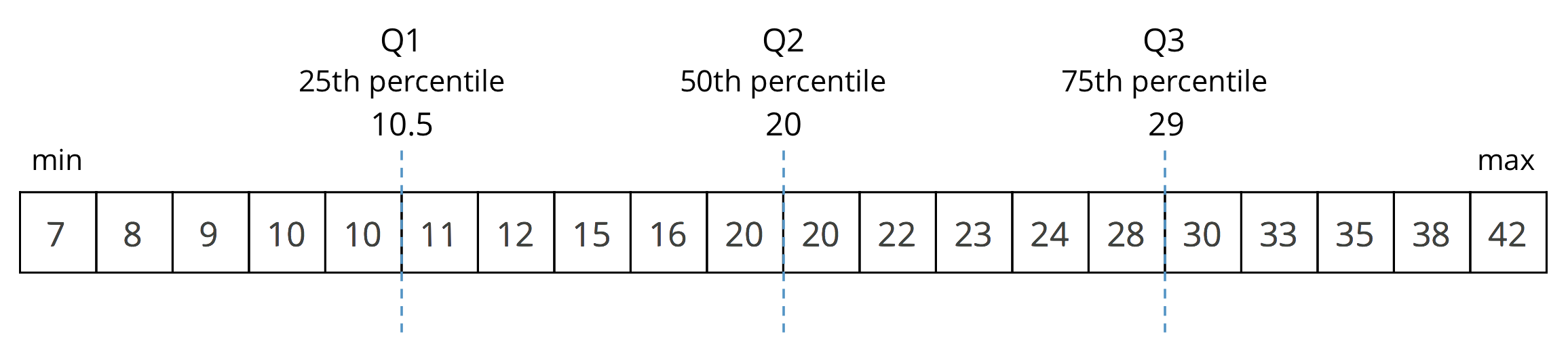
Ask a student to display the data set they have decomposed and labeled, or display the following image for all to see.
Focus the conversation on students' interpretation of the five numbers. Discuss:
- “In this context, what do the minimum and maximum values tell us?” (The ages of the youngest and oldest partygoers.)
- “Why are Q1 called 25th percentile, Q2 50th percentile, and Q3 75th percentile?” (Each quartile tells us how many quarters of the ordered data values are accounted for up to that point. The first quartile tells us that one quarter, or 25 percent, of data values are less than or equal to that value. The second quartile tells us that two quarters, or 50 percent, of data values are less than or equal to that value, and so on.)
- “In this context, what does Q1 (10.5) tell us?” (That a quarter of the partygoers are 10.5 years old or younger.)
- “What does Q3 (29) tell us?” (That three quarters of the partygoers are 29 years old or younger.)
- “How do the five numbers help us to see the distribution of the data?” (It divides the values in the data into sections containing one fourth of the values each. This gives us an idea about the distribution of the data by looking at how varied each section is.)
Supports accessibility for: Visual-spatial processing
Design Principle(s): Support sense-making
15.3: Range and Interquartile Range (15 minutes)
Activity
In the previous activity, students learned about the five-number summary and how it could be used to summarize a data set. Here, students extend their work to finding the range and interquartile range (IQR) of a data set. They learn that both values provide information about a distribution of data: the range is the difference between the maximum and minimum values in the data, while the IQR is the difference between the third and first quartiles. While the range tells us how spread out (or close together) the overall data values are, the IQR tells us how spread out (or close together) the middle half of the data values are.
Students identify the range and IQR of a data set and analyze distributions with different IQRs. They reason abstractly and quantitatively (MP2) as they use the IQR to describe the variability of data.
Launch
Tell students that they will write the five-number summary of a distribution shown on a dot plot. Give students a moment of quiet time to look at the dot plot in the first question and think about how they might identify the quartiles. Then, ask students to share their ideas. Students might suggest the following strategies.
- List the values of all the data points, put them in order, and then count off the values to find the median and the other two quartiles.
- Count the points by 3's (because the data set is to be decomposed into 4 equal parts and \(12\div 4=3\)) and mark the end of the first set with Q1, the end of the second set with Q2, etc.
- Divide the points into two halves (by counting 6 points from the left or from the right), and then dividing each half into two halves.
It is not necessary that all of these ideas are brought up at this point, but if no students mentioned the first approach (listing all values), mention it. The concrete process of writing out all the values, in order, is likely to be accessible to most students. The list of values would also be familiar, as it would resemble the one in the preceding activity.
Arrange students in groups of 2. Give students 3–4 minutes of quiet work time for the first question, and 5–7 minutes to discuss their work with their partner and to complete the rest of the activity. Follow with a whole-class discussion.
Student Facing
-
Here is a dot plot that shows the lengths of Elena’s bus rides to school, over 12 days.
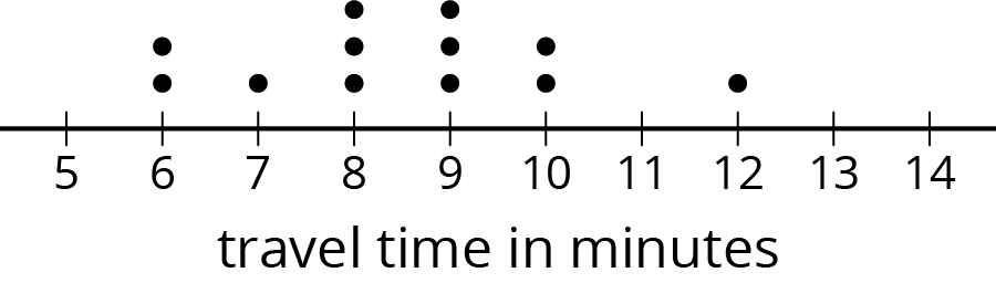
Write the five-number summary for this data set. Show your reasoning.
-
The range is one way to describe the spread of values in a data set. It is the difference between the maximum and minimum. What is the range of Elena’s travel times?
-
Another way to describe the spread of values in a data set is the interquartile range (IQR). It is the difference between the upper quartile and the lower quartile.
-
What is the interquartile range (IQR) of Elena’s travel times?
-
What fraction of the data values are between the lower and upper quartiles?
-
-
Here are two more dot plots.

Without doing any calculations, predict:
-
Which data set has the smaller range?
-
Which data set has the smaller IQR?
-
- Check your predictions by calculating the range and IQR for the data in each dot plot.
Student Response
For access, consult one of our IM Certified Partners.
Anticipated Misconceptions
When finding the IQR of the dot plots in the last question, students might neglect to divide the data set into four parts. Or they might instead divide the distance between the maximum and minimum into four parts (rather than dividing the data points into four parts). Remind students about the conversation at the start of the task about listing all the values or counting off the data points in order to find the quartiles.
Activity Synthesis
Ensure that students know how to find the range and IQR, and then focus the discussion on interpreting these two measures and how they provide information about a distribution.
Select a couple of students to share the range and IQR of Elena's data. Ask:
- “What does a range of 6 minutes tell us about Elena's travel time?” (Elena's travel times vary by 6 minutes at most, or that the difference between the shortest commute and the longest one is 6 minutes.)
- “What does an IQR of 2 minutes tell us about her travel time?” (The middle half of Elena's travel times vary by 2 minutes.)
Then, select a few other students to explain their response to the third question. Discuss:
- “Without calculating, how did you determine which data set had the smaller range?” (The dot plot that has the narrower spread would have the smaller range because the distance between the greatest and least values is smaller.)
- “How did you determine which one had the smaller IQR?” (The dot plot whose middle half of the points seem more clustered together would have the smaller IQR.)
- “In general, what does a larger range tell us?” (A wider spread in the data, more variability in the data set.)
- “What does a larger IQR tell us?” (A wider spread around the center of data, more variability in the middle half of the data set.)
- “Can a data set have a large range and a small IQR?” (It is possible, if the data set has most of its points very close together but there are a few points that are far away from the cluster.)
If not mentioned by students, explain that the IQR plays a similar role as the mean absolute deviation (MAD): it tells us how different and spread out the data values are. But instead of measuring the average distance of data values from the mean, it measures the span of the middle half of the data.
Supports accessibility for: Memory; Language
Design Principle(s): Support sense-making
Lesson Synthesis
Lesson Synthesis
- “What are the quartiles for a numerical data set?” (Numbers that show where we split the data up so it is in quarters.)
- “What is the relationship between the quartiles and the median?” (The second quartile is also the median).
- “What is the Interquartile range (IQR)? What does it mean?” (The IQR is the difference between the third and first quartile. It is a measure of the variability or spread of the data. It tells us how much “space” the middle half of the data occupies.)
- “Compare MAD and IQR. How are they alike? How are they different?” (They both provide information on the distribution of a set of data. MAD works with the mean while IQR works with the median. MAD considers all the data values and tells us the average distance between each data value and the mean, while IQR focuses on the middle half of the data and tells us how widely distributed it is.)
15.4: Cool-down - How Far Can You Throw? (5 minutes)
Cool-Down
For access, consult one of our IM Certified Partners.
Student Lesson Summary
Student Facing
Earlier we learned that the mean is a measure of the center of a distribution and the MAD is a measure of the variability (or spread) that goes with the mean. There is also a measure of spread that goes with the median. It is called the interquartile range (IQR).
Finding the IQR involves splitting a data set into fourths. Each of the three values that splits the data into fourths is called a quartile.
- The median, or second quartile (Q2), splits the data into two halves.
- The first quartile (Q1) is the middle value of the lower half of the data.
- The third quartile (Q3) is the middle value of the upper half of the data.
For example, here is a data set with 11 values.
| 12 | 19 | 20 | 21 | 22 | 33 | 34 | 35 | 40 | 40 | 49 |
| Q1 | Q2 | Q3 |
- The median is 33.
- The first quartile is 20. It is the median of the numbers less than 33.
- The third quartile 40. It is the median of the numbers greater than 33.
The difference between the maximum and minimum values of a data set is the range. The difference between Q3 and Q1 is the interquartile range (IQR). Because the distance between Q1 and Q3 includes the middle two-fourths of the distribution, the values between those two quartiles are sometimes called the middle half of the data.
The bigger the IQR, the more spread out the middle half of the data values are. The smaller the IQR, the closer together the middle half of the data values are. This is why we can use the IQR as a measure of spread.
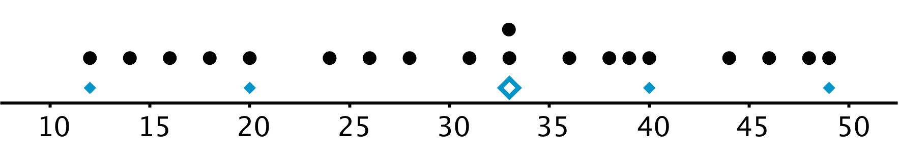
A five-number summary can be used to summarize a distribution. It includes the minimum, first quartile, median, third quartile, and maximum of the data set. For the previous example, the five-number summary is 12, 20, 33, 40, and 49. These numbers are marked with diamonds on the dot plot.
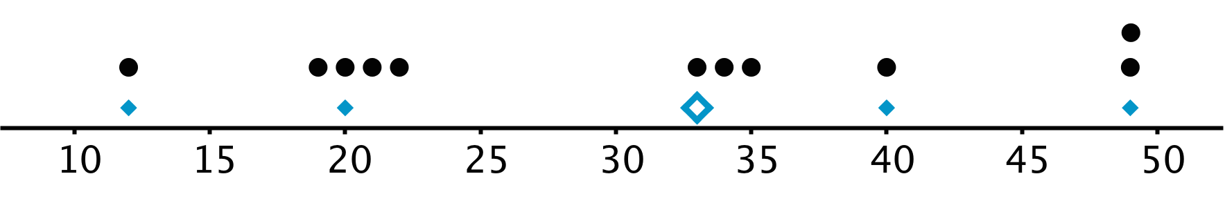
Different data sets can have the same five-number summary. For instance, here is another data set with the same minimum, maximum, and quartiles as the previous example.