Lesson 6
Residuals
- Let’s examine how close data is to linear models.
6.1: Math Talk: Differences in Expectations
Mentally calculate how close the estimate is to the actual value using the difference: \(\text{actual value} - \text{estimated value}\).
Actual value: 24.8 grams. Estimated value: 19.6 grams
Actual value: $112.11. Estimated value: $109.30
Actual value: 41.5 centimeters. Estimated value: 45.90 centimeters
Actual value: -1.34 degrees Celsius. Estimated value: -2.45 degrees Celsius
6.2: Oranges Return
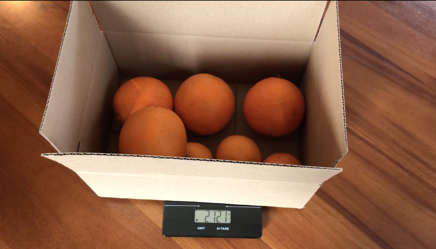
Use this data from the video about weighing oranges to answer the questions.
| number of oranges | weight in kilograms |
|---|---|
| 3 | 1.027 |
| 4 | 1.162 |
| 5 | 1.502 |
| 6 | 1.617 |
| 7 | 1.761 |
| 8 | 2.115 |
| 9 | 2.233 |
| 10 | 2.569 |
- Use technology to make a scatter plot of orange weights and find the line of best fit.
- What does the linear model estimate for the weight of the box of oranges for each of the numbers of oranges?
number of oranges actual weight in kilograms linear estimate weight in kilograms 3 1.027 4 1.162 5 1.502 6 1.617 7 1.761 8 2.115 9 2.233 10 2.569 - Compare the weights of the box with 3 oranges in it to the estimated weight of the box with 3 oranges in it. Explain or show your reasoning.
- How many oranges are in the box when the linear model estimates the weight best? Explain or show your reasoning.
- How many oranges are in the box when the linear model estimates the weight least well? Explain or show your reasoning.
- The difference between the actual value and the value estimated by a linear model is called the residual. If the actual value is greater than the estimated value, the residual is positive. If the actual value is less than the estimated value, the residual is negative. For the orange weight data set, what is the residual for the best fit line when there are 3 oranges?
- With digital technology, you can graph the residuals all at once. Check out the graph of the residuals. When graphed on the same axes as the scatter plot, what are the coordinates of the point where \(x = 8\) and \(y\) has the value of the residual?
- Which point on the scatter plot has the residual closest to zero? What does this mean about the weight of the box with that many oranges in it?
- How can you use the residuals to decide how well a line fits the data?
6.3: Best Residuals
- Match the scatter plots and given linear models to the graph of the residuals.
- Turn the scatter plots over so that only the residuals are visible. Based on the residuals, which line would produce the most accurate estimates? Which line fits its data worst?
-
Tyler estimates a line of best fit for some data about the mass, in grams, of different numbers of apples. Here is the graph of the residuals.

- What does Tyler’s line of best fit look like according to the graph of the residuals?
- How well does Tyler’s line of best fit model the data? Explain your reasoning.
-
Lin estimates a line of best fit for the same data. The graph shows the residuals.

- What does Lin’s line of best fit look like in comparison to the data?
- How well does Lin’s line of best fit model the data? Explain your reasoning.
-
Kiran also estimates a line of best fit for the same data. The graph shows the residuals.

- What does Kiran’s line of best fit look like in comparison to the data?
- How well does Kiran’s line of best fit model the data? Explain your reasoning.
- Who has the best estimate of the line of best fit—Tyler, Lin, or Kiran? Explain your reasoning.
Summary
When fitting a linear model to data, it can be useful to look at the residuals. Residuals are the difference between the \(y\)-value for a point in a scatter plot and the value predicted by the linear model for that \(x\) value.
For example, in the scatter plot showing the length of the fish and the age of the fish, the residual for the fish that is 2 years old and 100 mm long is 8.06 mm, because the point is at \((2,100)\) and the linear function has the value 91.94 mm (\(34.08 \boldcdot 2 + 23.78\)) when \(x\) is 2. The residual of 8.06 mm means that the actual fish is about 8 millimeters longer than the linear model estimates for a fish of that same age.
\(y = 34.08x + 23.78\)

When the point on the scatter plot is above the line, it has a positive residual. When the point on the scatter plot is below the line, the residual is a negative value. A line that has smaller residuals would be more likely to produce estimates that are close to the actual value.
Video Summary
Glossary Entries
- residual
The difference between the \(y\)-value for a point in a scatter plot and the value predicted by a linear model. The lengths of the dashed lines in the figure are the residuals for each data point.
